
Absolute Quantification with EvaGreen®
The increasing emergence and dissemination of antibiotic resistance (AR) is a threat to human and animal health worldwide. Organic solid waste including animal manure and sewage sludge from wastewater treatment plants has been recognized as rich reservoir of both antibiotic resistant bacteria (ARB), and antibiotic resistant genes (ARG). The common practice of soil fertilization with animal manure or municipal waste contributes to the dissemination of ARB and ARG in the environment. There is a growing interest in ecological studies of antibacterial resistance owing to the increasing concern over the potential risks associated with community-acquired infections as well resistance gene transfer, not only among commensals but also to pathogens.
Tracking microbes and their gene content requires sensitive and reliable methods. One of the technical challenges is to combine sensitivity, specificity, and universality (all gene sequences have to be detected at once). Digital PCR (dPCR) using EvaGreen® offers such potential.
Here we choose to report the detection of the ermB gene, encoding for erythromycin resistance, in various organic wastes exposed to a cleaning process involving digestion and composting using dPCR.
This antibiotic is used on both human and animal foods. The ermB gene (364 bp) encodes an rRNA methylase that hinders antibiotic binding to the ribosome and usually results in cross-resistance to macrolides, lincosamides, and streptogramins B antibiotics. It is the most widely distributed gene among the erm gene class. It is present in a variety of Gram-positive bacteria, including enterococci, streptococci, and staphylococci. The potential for inter-species horizontal gene transfer (HGT) has facilitated the emergence of resistance in multiple species including Gram-negative bacteria of the genera Bacteroides, Shigella, Escherichia, Klebsiella, and Campylobacter.
Data presented in this tutorial has been obtained in collaboration with Dr. Nazaret Sylvie from UMR 5557 Ecologie Microbienne, CNRS, INRA, VetagroSup, UCBL, Université de Lyon, 43 Boulevard du 11 Novembre, F-69622 Villeurbanne, France.
Assay Design
How should I design this assay?
First of all, note that the rules for primers design are the same in qPCR and digital PCR.
During the PCR, primers select the region of interest to be amplified. EvaGreen®, a green fluorescent dye, binds to the amplified double strand DNA and becomes highly fluorescent.
For more details, please see the Primers & Probes and PCR Basic Knowledge items.
Perform Experiment
What do I need to perform this experiment?
For any digital PCR experiment, you need:
- A digital PCR system and dedicated consumables
- PCR mastermix containing the polymerase, dNTPs (desoxyribonucleotides), etc. (please check manufacturer’s recommendations)
- 1 reference dye if necessary (please check manufacturer’s recommendations)
- Purified water
- General lab supplies for PCR: microfuge tubes, vortex, microcentrifuge, etc.,
Then for this specific experiment, you will need:
- 1 primer set to amplify the ermB gene class
- extracted DNA from various organic wastes
- EvaGreen®, if not already included in your ready-to-use master mix (please check manufacturer’s recommendations)
Primer sequences we used for this assay can be found in Chen, J., Yu, Z., Michel Jr, F. C., Wittum, T., Morrison, M. (2007). Development and Application of Real-Time PCR Assays for Quantification of erm Genes Conferring Resistance to Macrolides-Lincosamides-Streptogramin B in Livestock Manure and Manure Management Systems. Applied and Environmental Microbiology, 73(14), 4407-4416. doi:10.1128/AEM.02799-06
PCR Mix Preparation
How should I prepare my PCR mix?
Please note that this experiment has been done using the Naica™ System and the Sapphire chip.
a. Importance of DNA preparation
Once the DNA extraction has been done, you need to verify the DNA purity and quality of your samples.
For more details, please check the DNA preparation for Digital PCR item.
b. One more step before starting to manipulate: prepare your working sheet
If you are a qPCR user, the protocol for preparing the PCR mix is the same.
Here is what you need to know:
- how many samples do you want to run: for n=7 samples, in order to take into account the volume lost with pipetting error, prepare a total volume of PCR mix for n+1=8 samples.
- what are the manufacturer’s instructions for each component of the PCR mix?
Once you are ready, prepare your PCR mix as follows:
| Reagents | Final Concentration |
|---|---|
| PCR Mastermix (2X or 5X) | 1X or 0.75X, please refer to manufacturer’s instructions |
| Reference dye | Please refer to the manufacturer’s instructions |
| EvaGreen | Please refer to the manufacturer’s instructions |
| ermB primers | 200 nM |
| Organic Wastes DNA | unknown |
| Water | Up to 25 µL (depending on the manufacturer’s instructions) |
In this experiment, we will quantify the number of ermB copies in 1 NTC and 6 samples:
Initial wastes A and B (wastes to be cleaned) are sewage sludge and pig slurry samples, respectively.
Intermediate wastes A-1 and A-2 were sampled after the anaerobic digestion (A-1) and the composting (A-2) treatments of the initial waste A.
Final wastes A and B (cleaned wastes) were obtained after anaerobic digestion and composting process.
c. Everything is ready: the hands-on part!
Prior to preparing your PCR mix make sure you work in a clean area in order to avoid all sources of DNA contamination. The use of a PCR hood is recommended. Assemble the PCR mix based on your working sheet. Make sure all the components are well homogenized before loading the PCR mix into the consumables used for partitioning.
Finally, the hands-on protocol will vary according to your digital PCR system. Please check the manufacturer’s instructions. If you are using the Naica™ System (Stilla Technologies) or the QX200™ Droplet Digital™ PCR System (Bio-Rad), you can check the “Performing Digital PCR Hands-On” item.
Get Results
What steps are required to get my results?
a. Thermocycling
The ermB assay used in this example was optimized using the PerfeCTa qPCR ToughMix UNG mastermix on the Naica™ System (Stilla Technologies). In the table below you will find the thermocycling program used for the assay. If you are using a different mastermix or digital PCR system, you may have to optimize this protocol. For more details, please check “Digital PCR assay optimization” item.
| Cycles | Temperature | Time |
|---|---|---|
| 1 | 95 °C | 5 min |
| 5 | 94°C | 30 s |
| 63°C-59°C (Touchdown-1°C each cycle) | 30 s | |
| 72°C | 30 s | |
| 45 | 94°C | 30 s |
| 58°C | 30 s | |
| 72°C | 30 s |
Table 2: ermB assay cycling conditions. This program has been developed on a qPCR platform and directly transferred on the Naica™ System. Touchdown PCR increases the specificity of the PCR reaction.
b. Data Acquisition
Depending on the system used, data acquisition will take the form of imaging a chip (Naica™ System, QuantStudio™ 3D Digital PCR System, CONSTELLATION® digital PCR system, etc.), or reading partitions one-by-one in a process analogous to flow cytometry (QX200™ Droplet Digital™ PCR System, Raindrop™ Digital PCR System). Please follow manufacturer’s instructions on how to perform this step.
Analyze Data
How should I analyze my data?
In an EvaGreen digital PCR experiment, you have only one fluorescence channel to check so your data will be represented as a 1D dot-plot (Figure A).
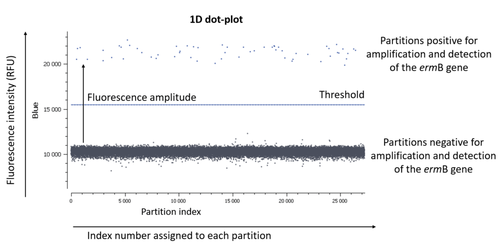
Figure A: The usual visualization of data in EvaGreen digital PCR experiments is by using a 1D dot-plot, in which each dot represents one partition. The y-axis gives the fluorescence intensity of each partition in the blue detection channel, while the x-axis gives the index number assigned to each partition by the analysis software.
For more details, please check the Fluorescence considerations with Evagreen® dye item.
a. Quality controls
Depending on the type of data acquisition, data analysis software can present different quality controls. Two criteria should be carefully considered:
- Check the NTC: none or very few positive partitions are accepted. As you can see in Figure D, our NTC presents only negative partitions.
- Check the total number of analyzed partitions: a high number of analyzable partitions will allow you to decrease the uncertainty associated with the measured concentration. In this assay, as you can see in table 3, we finally obtained between 25998 and 28269 partitions allowing us to validate our experiment.
On the Naica™ System, you can also visualize the generated partitions within the well. This will allow you to:
- Verify that the positive partitions are randomly distributed and thus, follow a Poisson distribution
- Verify the appearance of the partitions (size, level of fluorescence,etc.)
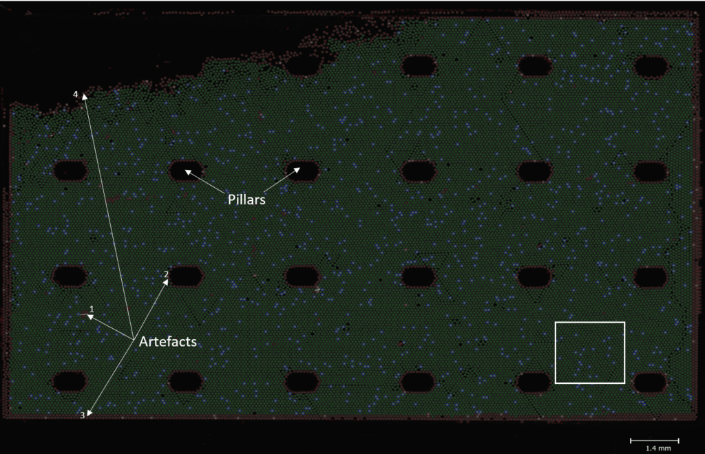
Figure B: Using the analysis software included in the naica® System, you can visualize the generated partitions for each sample. These partitions are self-assembled in a 2D monolayer array. The well is here called “chamber” and the pillars maintain its structure. The area in the top left corner appears empty: in order to avoid stacking, partitions do not completely fill the chamber. Three colors are used to distinguish artifacts (red crosses) from negative (green crosses) and positive (green crosses surrounded by blue circles) partitions. Artifacts are automatically excluded from the analysis. It can correspond to impurities like dust on the surface of the chamber (1). Partitions distributed around pillars (2) and the chamber (3) might be affected by the “edge effect” so the software identifies them as artifacts. Finally, isolated partitions (4) are also excluded. The white square represents the area presented in Figure B.
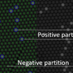
Figure C: Here, we zoomed in the area represented by a white square in Figure A. The legend can be removed so partitions can be easily visualized.
b. Threshold setting
Usually, the threshold is automatically set by the analysis software using a clustering algorithm that maximizes (resp. minimizes) inter-cluster (intra-cluster) point-to-point distances. Partitions above the threshold are positive and those under the threshold are negative. Thus, setting thresholds is a mandatory step to process to the quantification results by digital PCR.
Since the threshold setting is an automated calculation, we advise you to have a look at the dot-plots.
Indeed:
- when there is a very small number of positive partitions or a very small number of negative partitions, automated thresholding tends to fail out. Thus, the threshold has to be manually set
- when you observe a lot of partitions between the positive and the negatives ones (a phenomenon called “rain”), you might have to adjust the threshold as well (please note that you should also consider optimizing your assay if the rain is really important)
In this experiment, the threshold has been correctly set by the analysis software (Figure D).
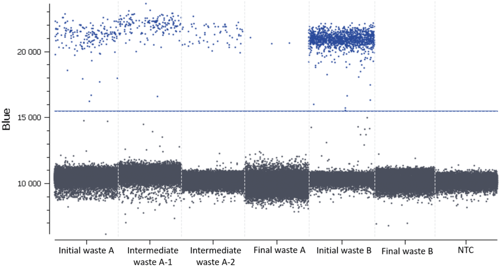
Figure D: 1D dot-plots for all tested samples and the NTC. The threshold is represented by a blue line. The negative and positive partitions are clearly separated so the analysis software was able to correctly set the automated threshold.
c. Calculating target concentration
The threshold being set, the software automatically quantifies the number of positive and negative partitions for each target. This digital readout is then converted to a result in the number of copies of the target per microliter using the Poisson distribution.
Each result is provided together with a 95% confidence interval which reflects the precision of the measurement. The accuracy of the measure can also be given by the “95% Confidence interval” value. The smaller, the better!
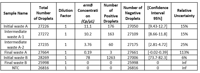
Table 3: For each sample concentration its 95% interval of confidence and its associated relative uncertainty is automatically calculated by the analysis software. Here, the dilution factor is 1 so the data obtained is the concentration in the well. Please note that if you prefer to obtain the concentration in your stock solution, do not forget to correct this value by your dilution factor.
In conclusion, data showed that both sewage sludge and pig slurry i.e. Initial wastes A and B, respectively, harbor ermB genes and that the cleaning processes led to the complete or almost complete elimination bacteria carrying this gene.
Summary
- Simply assay your samples with the conditions set up above, or optimized conditions if using another digital PCR system.
- Make sure you follow the MIQE guidelines if you are designing your own assay (For more details, please see the “MIQE Guidelines” item.)
- Verify that the threshold is placed adequately on your dot-plots.
- Export your results from the manufacturer’s software, making sure to include for each sample: the partition volume, the total number of partitions, as well as the number of positive partitions.
Congratulations for successfully following this digital PCR experiment!
Want to discover more dPCR experiments?
Check out our other tutorials!