
Introduction
The major advantages of digital PCR are its precision, sensitivity, and accuracy.
Indeed, digital PCR will enable you to detect and quantify rare mutations, even when present in very low amounts: less than 1% or even 0.1% of the wild-type (WT) sequence. Thus, for the detection and quantification of rare events, such as point mutations or single nucleotide polymorphism (SNP), digital PCR is the right tool for you!
In this tutorial, we will help you to prepare and analyze a rare mutation detection experiment from A to Z.
We choose here to focus on the detection of mutations occurring on the epithelial growth factor receptor (EGFR) gene. In patients with advanced EGFR-mutant non-small cell lung cancer (NSCLC), the presence of the mutation EGFR T790M renders the standard treatment, based on first and second-generation tyrosine kinase inhibitors (TKIs), ineffective. The EGFR T790M mutation is rarely detected during the initial tumor characterization and will, most often, become detectable over the course of treatment with TKI. Thus, early detection of the appearance of this mutation is of clinical importance in directing the patient to a more effective treatment.
Assay Design
How should I design an assay to detect a rare mutation?
First of all, note that the rules for designing probes and primers are the same in qPCR and digital PCR.
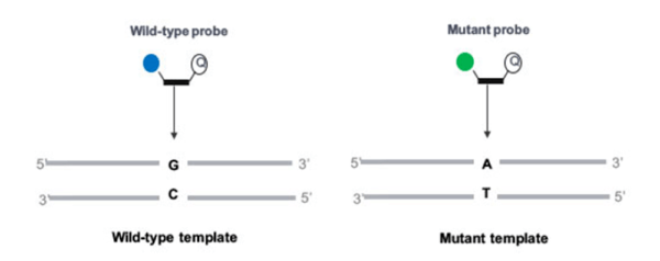
The option we have chosen here is to use two different hydrolysis probes (TaqMan®), with only one set of primers. These primers will amplify the region of interest. Then one probe, labeled with a specific fluorophore (represented as a solid blue circle in figure 1), will target the wild-type, and the other one, labeled with another specific fluorophore (represented as a solid green circle in figure 1), will target the mutant allele. Before ordering your probes, please check that the fluorophores you want to use are compatible with your digital PCR system in terms of excitation and emission spectra.
Finally, according to the principles of the hydrolysis probes, you will observe the generation of a fluorescent signal when the target sequence (mutant or wild-type) is present.
Perform Experiment
What do I need to perform a rare mutation detection experiment?
In addition to all the tools you would require for a standard PCR experiment (microfuge tubes, vortex, microcentrifuge, pipettes, and tips, etc.), for a digital PCR experiment you will need :
- A digital PCR system and its dedicated consumables
- A PCR mastermix (please check instrument manufacturer’s recommendations) containing all the essential components to perform an experiment, including:
- A DNA polymerase
- dNTPs (desoxyribonucleotides)
- reaction buffer
- MgCl2
- and nuclease-free water
- A reference dye if necessary (please check instrument manufacturer’s recommendations)
Then you will need for this specific experiment:
- 1 primer set to amplify the EGFR T790 locus
- 1 FAM-labeled hydrolysis probe to detect EGFR WT sequence
- 1 Cy3-labeled hydrolysis probe to detect EGFR T790M mutation
- WT DNA
- DNA bearing the EGFR T790M sequence
The primer and probe sequences we used for this assay can be found in [Madic, J., Zocevic, A., Senlis, V., Fradet, E., Andre, B., Muller, S., Dangla, R., Droniou, M.E. Three-color crystal digital PCR. Biomol Detect Quantif. 2016 Nov 3;10:34-46. eCollection 2016 Dec.]
PCR Mix Preparation
How should I prepare my PCR mix?
Please note that the following protocol has been optimized on the Naica™ System and the Sapphire chip.
a. Importance of DNA preparation and DNA input
Once your DNA has been extracted and purified, you have to calculate the amount of DNA you need to put in your reaction. This will determinate the sensitivity of your assay.
To do so remember in digital PCR we speak in terms of copies of DNA. The following formula will allow you to make the conversion:
Number of copies in reaction volume = mass of DNA in reaction volume (in ng)/0.003
Why 0.003? In this experiment, we are working with human genomic DNA: its mass is approximately 3 pg (=0.003 ng) per haploid genome, and we want to detect the EGFR gene which is present as one copy per haploid genome. If you are working with plasmids or other genomes, you will need to change this value.
Let’s do the math together with the following example, and you will understand how DNA input and sensitivity are related:
- Let’s say that we are working with a DNA input of 10ng (V = 1µL). With the Naica™ System and the Sapphire chip, the total PCR mix volume recommended is 25µL. By applying the formula in the section above, we can say that we are adding: 10/0.003 = 3,333 haploid genomes or copies of EGFR to our mix, meaning 3,333/25 = 133 copies of EGFR/µL as final concentration in the reaction well.
- Depending on the system used, the theoretical limit of detection may vary. With the Naica™ System, the lowest concentration theoretically detectable (theoretical LOD) with 95% confidence level is 0.2 copies/µL.
- Thus, to calculate the lowest theoretical sensitivity for this given sample with 95% confidence interval, we simply divide the theoretical LOD of the system by the total concentration of EGFR copies in our sample: Sensitivity = 0.2/133 = 0.15 %
In conclusion, with 10ng of human genomic DNA in your well and when using a digital PCR system with a 0,2 copies/µL theoretical LOD, you should be able to detect a mutated allelic fraction for EGFR down to 0.15 % with 95% confidence, but not lower.
For more details, please check “DNA preparation for Digital PCR” and “Digital PCR assay optimization” items.
b. One more step before starting to manipulate: prepare your working sheet
If you are a qPCR user, the protocol for preparing the PCR mix is the same.
Here is what you need to know:
- How many samples do you want to run: for n=7 samples, in order to take into account volume lost with pipetting error, prepare a total volume of PCR mix for n+1=8 samples.
- What are the manufacturer’s instructions for each component of the PCR mix
Once you are ready, prepare your PCR mix as follows:
Table 1: PCR mix
| Reagents | Final Concentration |
|---|---|
| PCR Mastermix (2X or 5X) | 1X |
| Reference dye | Please refer to the manufacturer’s instructions |
| EGFR T90 Reverse and Forward primers | 500 nM |
| EGFR T790WT probe | 250 nM |
| EGFR T790M probe | 250 nM |
| Human genomic DNA | ”How much DNA input”, see above |
| Water | Up to 25 µL (depending on manufacturers) |
Depending on the type of digital PCR system you are using you may have to generate a compensation matrix, i.e., monocolor controls. In this case, we are performing a duplex assay. Thus, you will need:
- 1 x Non-Template Control (NTC): in this well, you will put all the components of your PCR mix except DNA
- 1 x Monocolor control for EGFR T790WT probe
- 1 x Monocolor control for EGFR T790M probe
This will allow you to correct the fluorescence spillover that may occur between the two fluorophores. Please check the “Fluorescence spillover compensation” item for more details.
In this experiment, we will evaluate the presence of the T790M mutation in 4 samples.
c. Everything is ready: hands-on part!
Prior to preparing your PCR mix make sure you are working in a clean area in order to avoid all sources of DNA contamination. The use of a PCR hood is recommended. Assemble the PCR mix based on your working sheet. Make sure all the components are well homogenized before loading the PCR mix into the consumables used for partitioning.
Finally, the hands-on protocol will vary according to your digital PCR system. Please check the manufacturer’s instructions. If you are using the Naica™ System (Stilla Technologies) or the QX200™ Droplet Digital™ PCR System (Bio-Rad), you can check the “Performing Digital PCR Hands On” item.
Get Results
What are the next steps to get my results?
a. Thermal cycling
The EGFR assay used in this example was optimized using the QuantaBio PerfeCTa Multiplex mastermix, on the Naica™ System (Stilla Technologies). In the table below, you will find the thermal cycling program used for the assay. If you are using a different mastermix or digital PCR system, you may have to optimize this protocol. For more details, please check “Digital PCR assay optimization” item.
Table 2: EGFR T790M assay cycling conditions
| Cycles | Temperature | Time |
|---|---|---|
| 1 | 95°C | 10 min |
| 45 | 95°C | 30 s |
| 62°C | 15 s |
b. Data acquisition
Depending on the system used, data acquisition will take the form of imaging a chip (Naica™ System, QuantStudio™ 3D Digital PCR System, CONSTELLATION® digital PCR system,etc.), or reading partitions one-by-one in a process analogous to flow cytometry (QX200™ Droplet Digital™ PCR System, Raindrop™ Digital PCR System). Please follow manufacturer’s instructions on how to perform this step.
Analyze Data
How should I analyze my data?
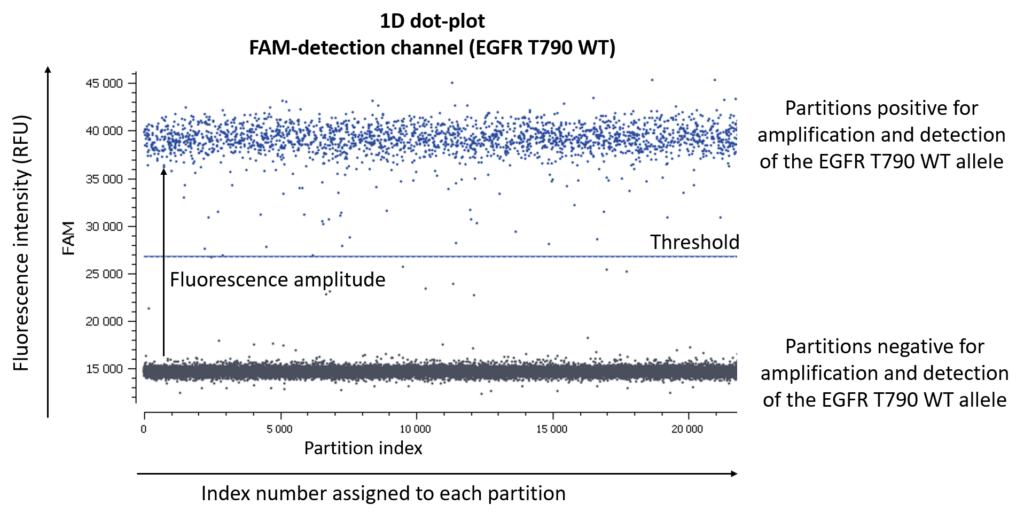
First of all, let us remind you of the usual graphical representation in digital PCR experiments are 1D-, 2D-, or 3D-dot-plots depending on the number of targets you are looking for.
If you are looking for 3 different targets, a 3D dot-plot graph will allow you to visualize the different clusters in the 3D space.
a. Quality controls
Depending on the type of data acquisition, data analysis software can present different quality controls. Two criteria should be carefully considered:
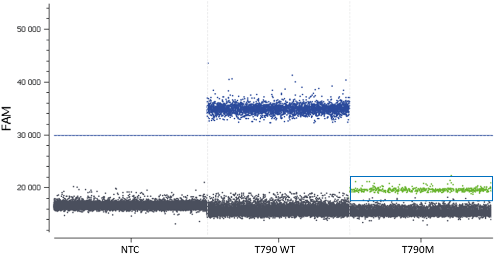
- Check the NTC, any or very few positive partitions are accepted. As you can see in figure 4, our NTC presents only negative partitions
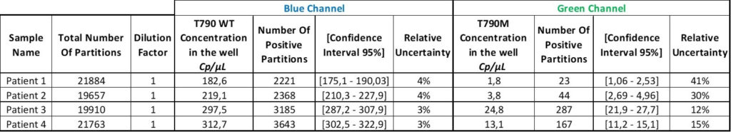
- Check the total number of analyzed partitions. Since we are looking for a rare mutation, we can say “the more, the better”. Indeed, with a high number of analyzable partitions, you increase the chance to detect and quantify a rare event, and you decrease the uncertainty associated with the measured concentration. In this assay (table 3) we obtained between 19,000 and 22,000 partitions, validating our experiment
b. Spillover compensation: not available on all digital PCR platforms
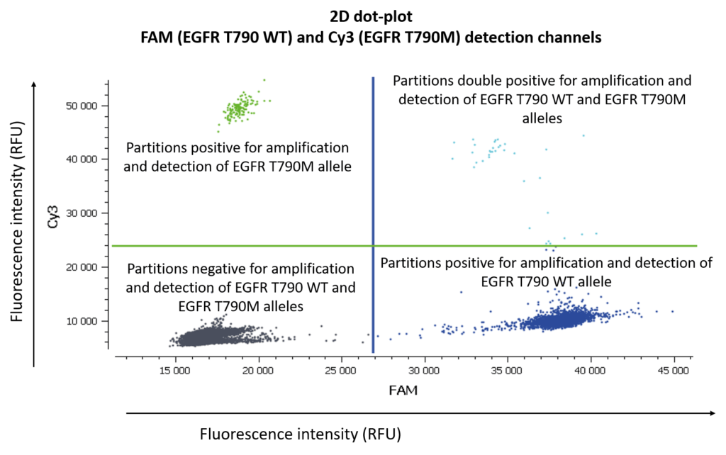
When performing multicolor digital PCR experiments, you may encounter fluorescence spillover. This physical phenomenon may be misleading and may yield aberrant results. Thus, you must apply a compensation matrix to the results.
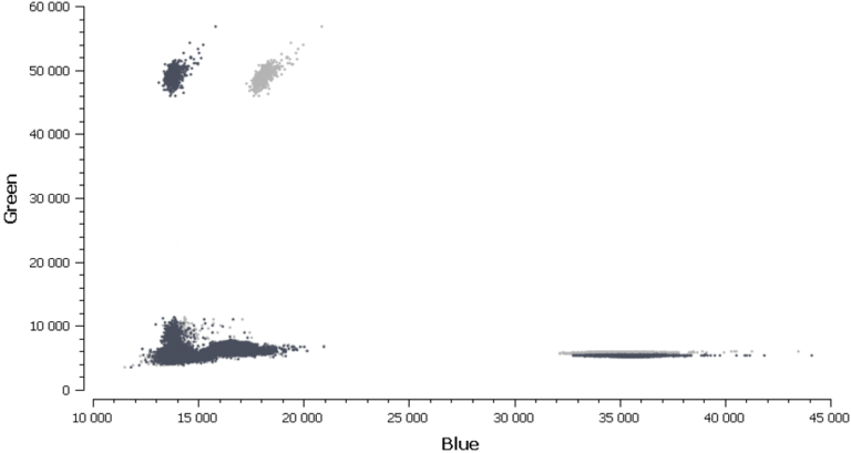
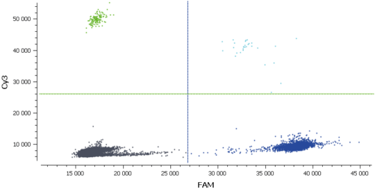
In figure 3, Cy3 fluorescence (coming from EGFR T790M probe), normally detected in the green channel, is causing a second cluster in the Blue channel because Cy3 is partially excited by the blue light source. You can also expect to visualize the detection of the FAM fluorescence (coming from the EGFR T790WT probe and normally detected in the blue channel), in the green channel because FAM is partially excited by the Green source. In figure 5, we can also observe a non-orthogonal disposition of the clusters on the 2D dot-plot. By indicating the wells containing monocolor controls to the software, the matrix compensation will be automatically generated and can be applied to your data.
Once the fluorescence spillover has been corrected, we can proceed to the next step- analysis of patient samples.
c. Threshold setting
Usually, the threshold is automatically set by the analysis software using a clustering algorithm that maximizes (resp. minimizes) inter-cluster (intra-cluster) point-to-point distances. Partitions above the threshold are positive and those under the threshold are negative. Setting the threshold is thus, a mandatory step to process and accurately quantify the samples.
Since the threshold setting is an automated calculation, we advise you to have a look at the dot-plots.
Note:
- When there are a very small number of positive partitions or a very small number of negative partitions, the threshold has to be manually set.
- When you observe a lot of partitions between the positive and the negatives ones (a phenomenon called “rain”), you might have to adjust the threshold (please note that you might also consider optimization of your assay if the rain is really important).
- When there is a cross-reactivity between probes, you can observe more clusters than expected. Make sure that these clusters are not coming from fluorescence spillover, by applying the compensation matrix if the software offers this option. Then, according to the result obtained, adjust the threshold.
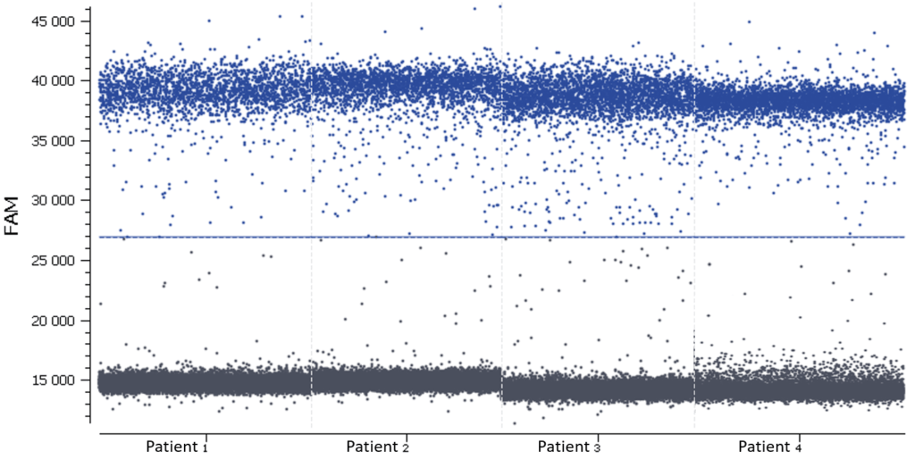
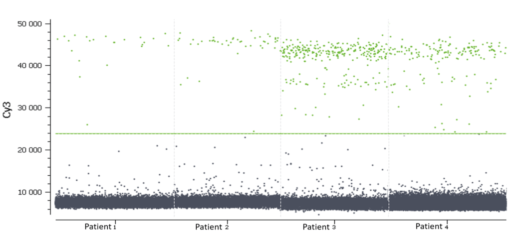
In this experiment, the threshold has been correctly set by the analysis software (figures 6, 7). For more details, see the Advanced Threshold Setting item.
d. Calculating target concentration
After the correct threshold setting, the software automatically quantifies the number of positive and negative partitions for each target. This digital readout is then converted to a result displayed as the number of copies of the target per microliter using the Poisson distribution.
Thanks to the Poisson distribution, each result will be provided together with a 95% confidence interval which reflects the precision. The accuracy of the measure can also be given by the “95% Confidence interval” value. The smaller, the better!
We now have the result table of the experiment but this does not mean that the analysis is done!
e. Calculating the Limit of Blank and Limit of Detection
For each new assay the Limit of Blank (LOB) and the Limit of Detection (LOD) must be estimated- not only prior to routinely using your assay, but also every time you change your assay as a part of its validation. This step will ensure unbiased results.
Why should I evaluate the LOB? In rare mutation detection assays, sometimes false positives are encountered, i.e. positive partitions for the mutated allele although the sample contains only wild-type templates. In other words, “noise” of the assay. In general, false positive partitions can be due to non-specific hybridization of the mutant probe onto wild-type sequence, polymerase error, well-to-well contamination, environmental contamination, template degradation, or base substitution due to template degradation. The false positive rate is assay dependent. Ideally, it should be zero but false positives can be very difficult to completely get rid of. To evaluate a statistically relevant LOB it is necessary to perform the assay on more than 30 wild-type controls.
For more details about LOB calculation, see the item below about LOB & LOD Definition.
Why should I evaluate the LOD? The LOD is a theoretical value representing the lowest concentration of detectable target in a well with 95% confidence. The larger the LOB, the larger the LOD for your assay.
For more details about LOD calculation, see the item below about LOB & LOD Definition.
The LOB is most frequently expressed as the number of positive partitions within a well. Let’s assume that we are working on an assay for which the LOB is estimated to be 4 positive partitions. After running the assay positive samples are obtained and one of them exhibits 3 positive partitions. In this case, the target is said to be “not detected with 95% confidence level” because it is not possible to say whether the positive signal is from the false positives (noise) or the actual targets present in the sample (signal).
In the EGFR T790WT/M assay, we assayed 32 samples containing WT DNA and calculated the frequency of positive partitions in these samples. Using the LOB calculator tool below, we found that the LOB for this assay was 2 partitions.
Now that you have the LOB, you can assay your samples and detect the EGFR T790M mutation with a 95% confidence level only if the number of positive partitions found in your samples is strictly larger than your LOB. Simply use the online calculators to get a lower-bound estimate of the real concentrations for each sample (Table 4).
The results for rare mutation detection are usually presented in terms of VAF (Variant Allele Frequency), or the percentage of mutation. If the analysis software does not have the option for a VAF result, you can use this VAF calculator.
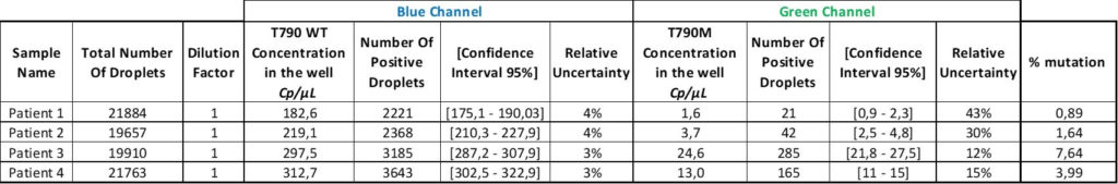
Finally, in the last column, the VAF for each sample was calculated using the formula “VAF = (Cmut/(Cmut+CWT))”
Finally, the last column of the table shows the percentage of mutation for each patient. The oncologists can adjust the treatment based on these results.
LOB and LOD Definition
Before routinely using your digital PCR assay, you should estimate the Limit Of Blank (LOB) and the Limit Of Detection (LOD).
Starting with the LOB, the estimation of the LOD will be then derived from this estimated LOB.
How would you define each parameter?
When the number of positive partitions found in a sample is:
- smaller than the LOB, then the target is said not detected
- larger than the LOB, then the target is said detected
Here are the mathematical definitions of LOB and LOD :
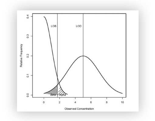
- The Limit of Blank 𝐿𝑂𝐵LOB with a confidence level (1–𝛼)(1–α) is defined (in number of partitions) as the maximum number of positive partitions expected in a well with a probability of 1–𝛼1–α in a sample containing no target sequence.
In other words, it is the maximum number of false positives that are plausible with a 1–𝛼1–α probability (typically 95% for 𝛼=5%α=5% of false positives).
- The Limit of Detection 𝐿𝑂𝐷LOD with a confidence level (1–𝛽)(1–β) is defined as the minimum concentration for which detecting the target sequence in a well is possible with a probability of 1–𝛽1–β.
In other words, this is the minimum concentration that can be said to be non-zero and statistically higher than the limit of blank 𝐿𝑂𝐵LOB with a 1–𝛽1–β probability (typically 95% for 𝛽=5%β=5% of false negatives).
Summary
- Assay your samples with the conditions set up as described above, or using optimized conditions if using another digital PCR system.
- Check that any fluorescence post-treatment corrections such as spillover compensation are performed.
- Verify that the thresholds are placed adequately on the dot-plots.
- Export results from the manufacturer’s software, making sure to include for each sample: the partition volume, the total number of partitions, as well as the number of positive partitions.
- Subtract the number of partitions found for the LOB from the number of positive partitions in the samples.
- Use online calculators to recalculate the corrected concentrations for each sample.
Congratulations on successfully performing this digital PCR experiment!
Want to discover more dPCR experiments?
Check out our other tutorials!